@misc{stenson2026infinity,
  author = {Trevor Stenson},
  title = {The Infinity Wheel: A Magnetically-Coupled Mechanical Oscillator with Algebraically-Designed Mass Asymmetry},
  year = {2026},
  url = {https://system9.ai/research/infinity-wheel-coupled-oscillator},
  howpublished = {\\url\{https://system9.ai/research/infinity-wheel-coupled-oscillator\}},
  note = {Draft, in preparation}
}

The Infinity Wheel: A Magnetically-Coupled Mechanical Oscillator with Algebraically-Designed Mass Asymmetry

Canonical master draft. Companion to the math paper at papers/math/canonical.md. Cites it as [Math2026] for mathematical foundations rather than re-deriving them. Target audience: engineering / physics journal-grade rigor. Derivative versions (engineering journal, maker writeup, README, whitepaper PDF) derive from this document. Version 0.1, first complete draft.

---

Abstract

We present the design and physical principles of a coupled mechanical oscillator consisting of two large vertical wheels (304.8 mm outer diameter), magnetically coupled along a fixed-gap axis to counter-rotate without physical contact. Each wheel carries 12 weight stations at 30° angular intervals, accommodating 0–9 half-ounce lead segments per station. The per-station weight counts are determined by the digital-root Fibonacci 24-cycle described in a companion mathematical paper [Math2026], producing the design property that opposing angular stations across the two wheels always sum to nine weights, except at one antipodal pair which sums to either 18 or 0, an experimental degree of freedom representing the two physical realizations of the same algebraic equivalence class.

The asymmetric mass distribution combined with magnetic synchronization produces standard Huygens-style coupled-oscillator behavior with rhythmic phase-locking. An earlier prototype demonstrated sustained oscillation under minimal frictional input (a held pencil sufficed as a low-friction axle) suggesting the design operates in a high-Q regime suitable as a physics demonstration. We describe the parametric CAD model (open-source Python via CadQuery), the choice of Multi Jet Fusion (MJF) PA12 as the print substrate, the bearing and magnetic-coupling specifications, and an open-source implementation that allows reproducing or modifying the design.

The device is a demonstration of the illusion of perpetual motion in the tradition of overbalanced wheels dating to Bhāskara II's Siddhānta-Śiromaṇi (12th century). It does not claim and does not produce energy from nothing. Standard coupled-oscillator analysis applies; observed dynamics are within the predictions of Newtonian mechanics with magnetic coupling and dissipation. The novelty is the algebraic derivation of the mass distribution (rather than ad hoc choices), and the resulting symmetry between the two coupled wheels.

---

1. Introduction

1.1 Background and motivation

Asymmetric-mass wheels designed to demonstrate the appearance of perpetual motion have a continuous history dating to Bhāskara II's overbalanced wheel (12th century) and persisting through Villard de Honnecourt (13th century), Leonardo da Vinci, and modern museum exhibits. None of these devices produces energy; all are bounded by the laws of thermodynamics and eventually decelerate under friction. They remain compelling as demonstrations because the asymmetric mass distribution can sustain rhythmic oscillation for long durations under low friction, producing what naïve observers experience as continuous motion.

Modern coupled-oscillator theory provides the framework for understanding such devices precisely. Huygens documented in 1665 that two pendulums sharing a slightly-compliant base will phase-lock: the original observation underlying today's Kuramoto-model treatment of synchronization phenomena across physics, biology, and chemistry [PRK01]. Magnetic gears, introduced as a contactless analog of mechanical gear trains [Atallah2001], offer one route to such coupling without sliding friction.

This paper describes the design of a device combining these elements:

• Two large (12-inch / 304.8 mm diameter) vertical wheels in a shared frame.
• Asymmetric mass distribution at 12 weight stations per wheel, with the per-station weight counts derived from the orbit structure of the digital-root Fibonacci recurrence described in a companion mathematical paper [Math2026].
• Magnetic coupling between the wheels via a ring of alternating-pole permanent magnets in each rim, producing 1:1 contactless counter-rotational coupling.
• Open-source parametric CAD implementation in Python (CadQuery), publishable via Multi Jet Fusion (MJF) PA12.

1.2 Contributions

The contributions of this paper are:

1. A specific design where the mass distribution is determined (rather than chosen ad hoc) by an underlying mathematical structure (the dr-Fibonacci 24-cycle) yielding the design property that opposing stations always sum to a constant (9 weights), with one antipodal exception that admits two physically valid configurations.

2. An open-source parametric CAD implementation (magnetic_gear/ in the accompanying repository) that allows the design to be reproduced, modified, and extended.

3. A coupled-oscillator analysis grounding the device's expected behavior in standard nonlinear dynamics, with the empirical observation that a v1 single-wheel prototype demonstrated the predicted high-Q regime.

1.3 Scope and what this paper does not claim

This is a physics demonstration, not a perpetual-motion device. The system is dissipative; oscillation is sustained only as long as input energy or stored momentum exceeds friction losses. The novelty here is in the design synthesis (algebraically derived mass distribution combined with magnetic coupling) not in any claim of new physics, free energy, or violations of thermodynamic conservation laws.

The mathematical structure that determines the mass distribution is interesting in its own right and is treated separately in the companion paper [Math2026]. The present paper assumes that paper as a reference and focuses on the engineering and physical principles of the device.

---

2. Background

2.1 Coupled mechanical oscillators and Huygens synchronization

A physical pendulum is any rigid body free to rotate about a horizontal axis under gravity. For a body with mass m and center of mass at distance r from the rotation axis, the restoring torque about the axis is

τ(θ) = -m g r sin(θ)

where θ is the angle of the line from axis to center of mass relative to vertical. For small angles, this linearizes to τ ≈ -m g r θ, giving simple harmonic motion with angular frequency ω = √(m g r / I) where I is the moment of inertia about the rotation axis.

Two such pendulums coupled by some mechanism (Huygens used a flexible wooden beam shared between two clocks) exhibit phase locking: their oscillations synchronize, generally in anti-phase for symmetric pendulums on a compliant base. The mathematical formalism for this is the Kuramoto model and its many extensions [PRK01]. The key parameters are the coupling strength K between the oscillators and any frequency mismatch Δω; for K > Δω, the oscillators lock into a fixed phase relationship.

The infinity wheel is a coupled-oscillator system in this sense, with two physical pendulums (the two weighted wheels) coupled by a magnetic-gear arrangement (§2.2).

2.2 Magnetic gears

A magnetic gear couples two rotating bodies through magnetic forces between permanent magnets embedded in each, without physical contact between gear teeth. The simplest configuration is two co-axial cylinders with alternating-pole magnets around their circumferences; magnets on adjacent cylinders attract or repel as the cylinders rotate, producing a torque coupling whose strength depends on the gap between cylinders and the magnetic field strength.

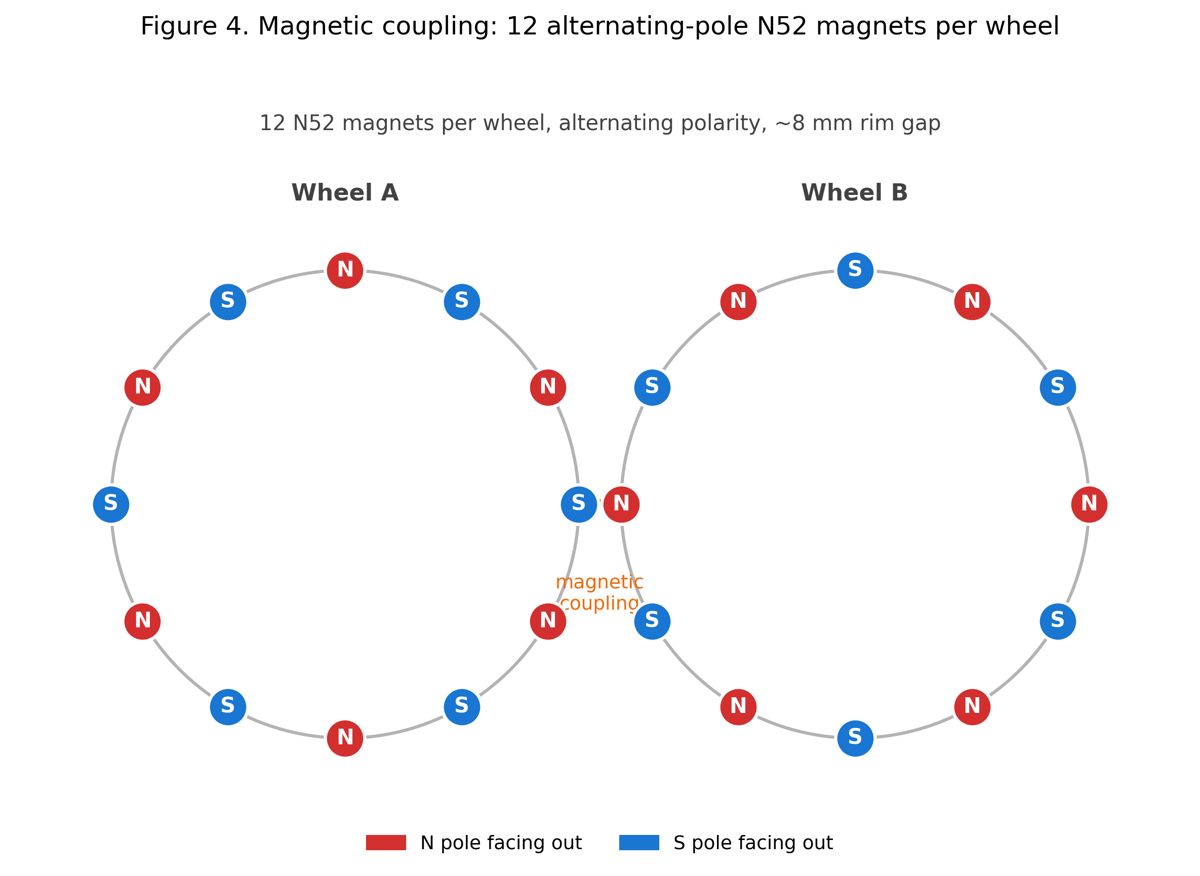
For the infinity wheel, we use a side-by-side (rather than co-axial) magnetic-gear arrangement: two wheels in the same plane with a small rim-to-rim gap, each wheel carrying 12 magnets around its outer rim with alternating polarity. As one wheel rotates, the magnets at its rim attract their counterparts of opposite polarity on the adjacent wheel, dragging the second wheel into counter-rotation. The 12-magnet-per-wheel configuration gives a 1:1 coupling ratio: one full rotation of wheel A produces one full rotation of wheel B, in opposite direction.

The magnetic-coupling literature gives precise expressions for torque vs. angle vs. gap for various magnet geometries [Atallah2001 and follow-up work]. For the present design, we operate well within the linear-coupling regime: the ~8 mm rim gap, 12 mm diameter × 4 mm thickness N52 magnets give peak coupling torques on the order of 0.5–1.0 N·m at the rim, far in excess of what is needed to couple the wheels' rotational dynamics.

2.3 Asymmetric-mass wheels: historical context

The design lineage of asymmetric-mass wheels demonstrating apparent perpetual motion includes:

• Bhāskara's wheel (12th century), a wheel with curved spokes containing mercury that supposedly remained out of balance throughout rotation. Documented in Siddhānta-Śiromaṇi.
• Villard de Honnecourt's wheel (~1230), a wheel with hammers swinging from its rim, intended to remain perpetually overbalanced.
• Leonardo da Vinci's wheel sketches, multiple variations in his notebooks.
• Modern museum demonstrations, notably at exhibits explaining why such devices cannot work (typically with rotation imparted externally and friction-bounded decay).

All of these share the design intuition that asymmetric mass + low-friction support produces sustained oscillation. None produces energy. The infinity wheel sits in this lineage with two distinguishing features: (1) the asymmetry pattern is derived from algebra (the dr-Fibonacci 24-cycle) rather than chosen ad hoc, and (2) the device couples two wheels magnetically rather than presenting a single wheel.

2.4 The mathematical foundation

The mass distribution is determined by the dr-Fibonacci recurrence and its orbit structure [Math2026]. We summarize the relevant facts here without re-deriving them:

• The recurrence xₙ = dr(xₙ₋₁ + xₙ₋₂) where dr is the digital root mod 9 (with 0 ↔ 9 convention) has Pisano period 24 in its second-order behavior [Math2026, §2.3].
• The space of starting pairs (a, b) ∈ Z₊² decomposes into exactly five orbits: three Hamiltonian length-24 cycles, one length-8 orbit on {3, 6, 9}, and the fixed point (9, 9) [Math2026, Theorem 3.1].
• Within each length-24 orbit, antipodal positions (separated by 12 indices) sum to 9, except one antipodal pair where both positions hold the value 9 (sum = 18), the "asymmetric self-mirror" or "9+9 special pair" [Math2026, Theorem 5.1].

These facts directly motivate the device geometry: 12 angular stations per wheel, two wheels carrying the two halves of a 24-cycle, with the antipodal pair-sum-to-9 property guaranteeing that opposing wheel-stations always have a constant total weight.

---

3. Design Rationale

3.1 Why 12 stations per wheel

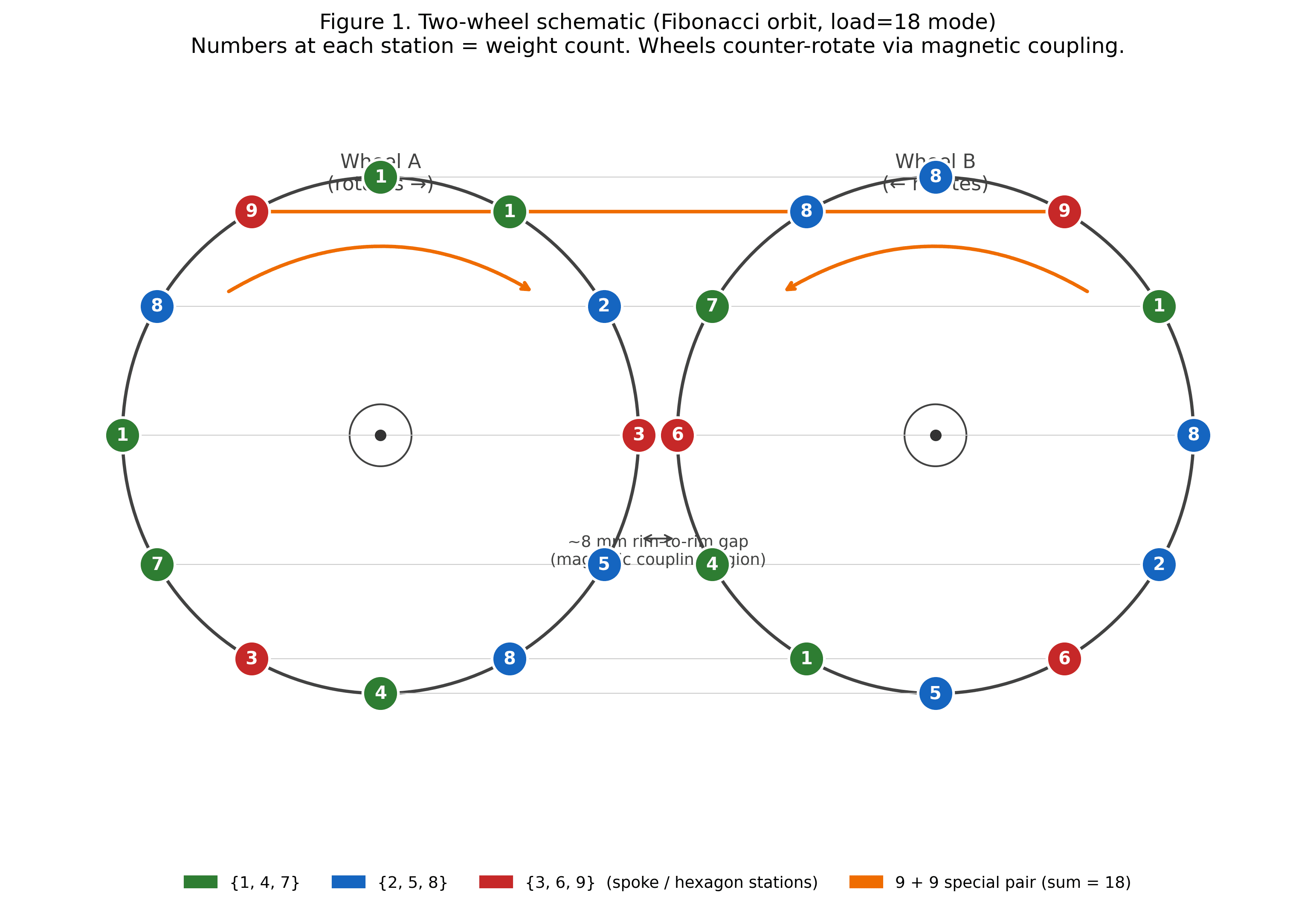
The dr-Fibonacci 24-cycle splits naturally into two halves of 12 elements each. By the antipodal involution [Math2026, Theorem 5.1], position i in the first half pairs with position i + 12 in the second half such that their values sum to 9 (or 18 at the special pair). Placing the first 12 values on Wheel A and the next 12 on Wheel B realizes this pairing physically: when the two wheels are aligned in their initial configuration, opposing stations always have weight-counts summing to a constant.

The choice of 12 stations per wheel is therefore not a design preference; it is dictated by the half-period structure of the algebra.

3.2 Why digital-root Fibonacci specifically

Any asymmetric weight distribution will produce a wheel that oscillates as a physical pendulum. The dr-Fibonacci-derived distribution is distinguished by the guarantee that opposing wheel-stations always sum to a constant (9). This constant-sum property has a direct physical consequence:

At every angular position of the coupled-wheel system, one wheel is heavier than the other by a deterministic amount of mass, varying only by which side is heavier as the wheels rotate.

This maximizes the consistency of the gravitational torque differential available to the coupled-oscillator dynamics. Random asymmetric distributions would produce variable instantaneous torque differentials at different angular positions; the dr-Fibonacci distribution makes the torque differential's mass-magnitude constant (modulo the 9+9 special pair), with only the direction changing as the wheels rotate.

We do not claim the dr-Fibonacci distribution is optimal in any quantitative sense; we claim it is algebraically distinguished and produces an aesthetically and structurally clean design. The math paper [Math2026] provides the theoretical basis; experimental comparison with other asymmetric distributions is left for future work.

3.3 The 9+9 special pair as design degree of freedom

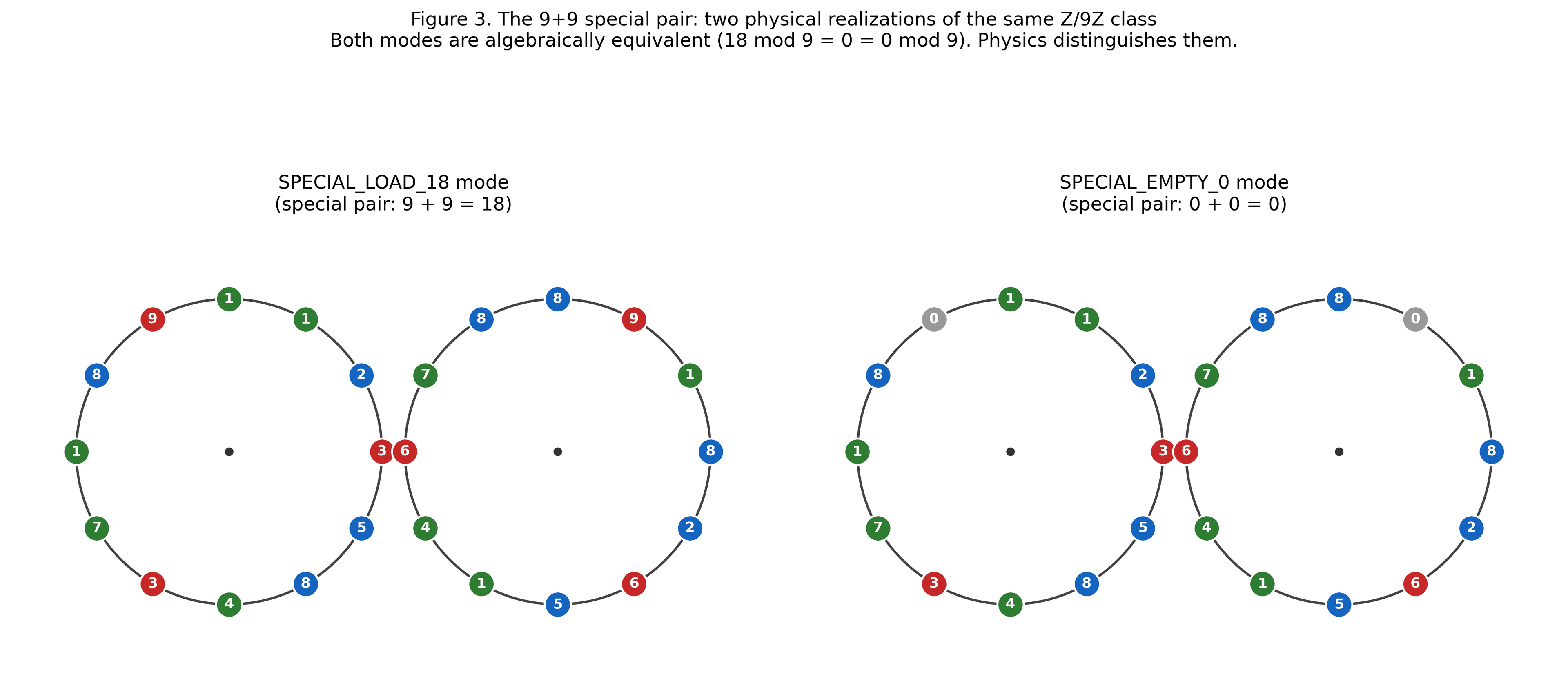
One antipodal station pair has both endpoints equal to 9, giving a physical sum of 18 weights. The math admits two realizations of this configuration, both representing the same Z/9Z residue class [Math2026, Remark 5.7 and §9.2]:

• SPECIAL_LOAD_18 (both special-pair stations loaded fully (9 weights each, total = 18). Maximum local mass) and torque differential, if any, concentrated at this single station.
• SPECIAL_EMPTY_0: both special-pair stations empty (0 weights each, total = 0). The asymmetric ring has a "void" patch at the special station, a balanced gap in the otherwise asymmetric circumference.

Both configurations are physically valid and mathematically equivalent (both reduce to the 0 ≡ 9 class in Z/9Z). Only the dynamics distinguish them: load=18 contributes maximum local imbalance at the special-pair angular position, while load=0 produces a gap in the imbalance pattern. The expected difference in oscillation behavior (frequency, sync stability, decay rate) is an empirical question.

The wheel design therefore preserves both modes as runtime-switchable configurations (SPECIAL_PAIR_MODE in params.py). The SPECIAL_PAIR_MODE constant is a deployment parameter, not a hardware change; the snap-cap pockets accommodate either configuration without rebuild. The physical-comparison experiment is a direct empirical probe of which physical representative of an algebraically equivalent class produces preferable coupled-oscillator behavior.

3.4 Three valid wheel pairings; one is built

The math identifies three length-24 orbits: O_F (seed (1, 1), the canonical Fibonacci), O_L (seed (1, 3), a Lucas-like sequence), and O_3 (seed (1, 4)) [Math2026, Theorem 3.1]. Each orbit corresponds to a distinct wheel pairing.

The build target for v2 is the Fibonacci orbit O_F. Its weight distribution is:

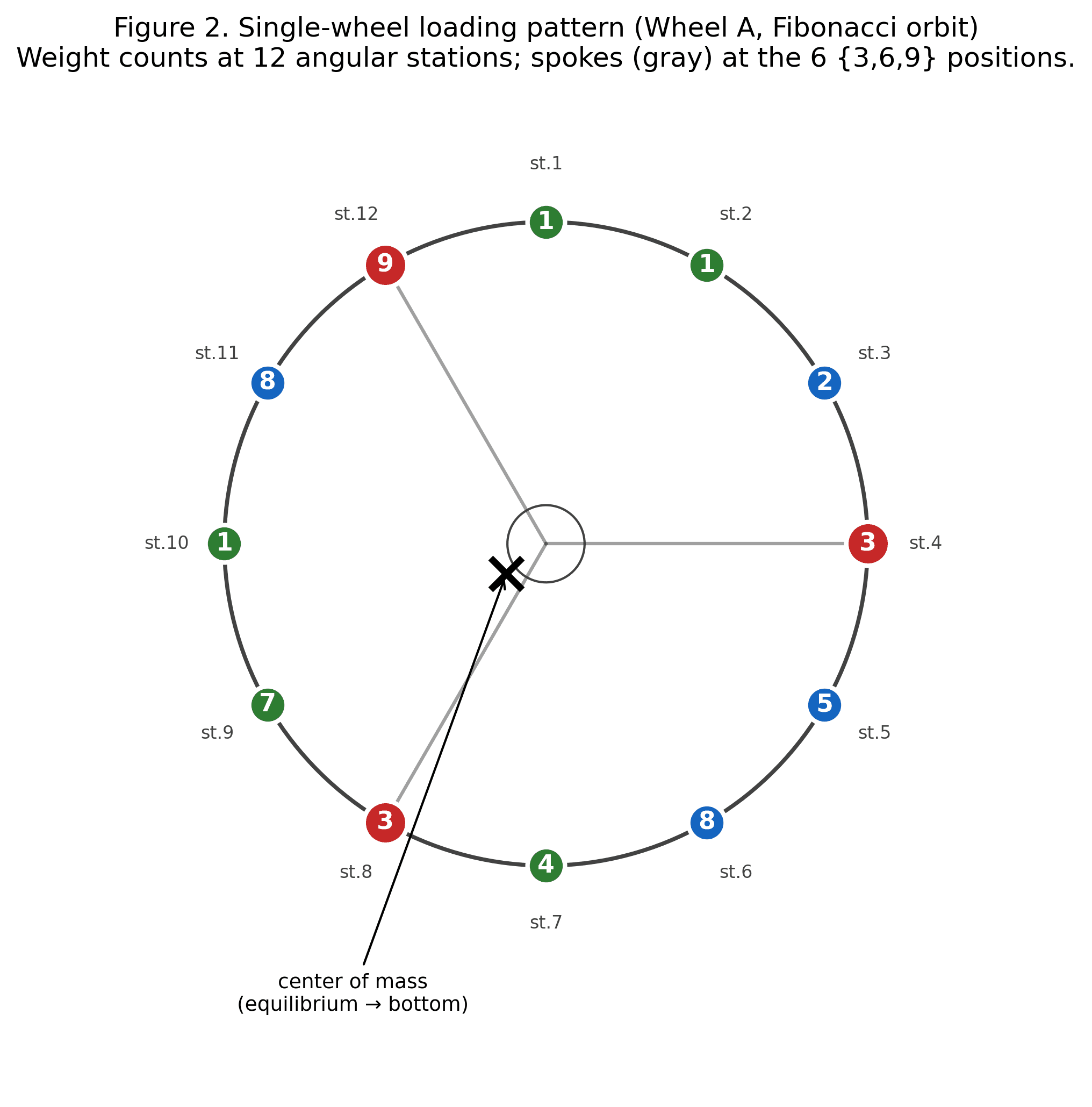
Wheel A (positions 1–12):   1, 1, 2, 3, 5, 8, 4, 3, 7, 1, 8, 9
Wheel B (positions 13–24):  8, 8, 7, 6, 4, 1, 5, 6, 2, 8, 1, 9

The other two orbits O_L and O_3 are reachable on the same hardware by reconfiguring weights according to their respective sequences. The hardware does not need to be rebuilt to test alternate orbits; configuration lives in the snap-cap pockets, not in the geometry.

3.5 The figure-8 topology: why the device is named the "Infinity Wheel"

The two-wheel device is the natural physical realization of an immersion of the 24-cycle into the plane as a figure-8 (lemniscate). In this immersion, the two 9-positions (which are antipodal in the cyclic order of the math paper [Math2026, §5.5]) coincide at a single central crossing. The two lobes of the figure-8 are the two physical wheels; the central crossing is the magnetic-coupling region where the wheels' rims meet.

This means the two wheels are not two separate objects; they are the two lobes of one continuous topological loop (the dr-Fibonacci 24-cycle), with the loop traversing itself at the magnetic-coupling region. The 9-9 special-pair station is permanently fixed at the crossing; every other station passes through the coupling region transiently as the wheels rotate. The cyclic structure has no preferred starting point or direction, the loop closes back on itself in the manner of the classical ouroboros (snake eating its tail), with the figure-8 crossing as the visible point of closure.

The name "Infinity Wheel" describes this exactly: the device is one infinity-sign-shaped loop, materialized as two coupled wheels.

3.6 Three independent design degrees of freedom

The design realizes a single abstract orbit through three independent design parameters [Math2026, §9.2]. All three are algebraically equivalent, switching any of them gives a different physical realization of the same abstract object:

Degree of freedom	Where set	Effect
(1) Orbit choice	params.py: ACTIVE_CONFIG	Which of the 3 length-24 sequences
(2) Rotational placement	physical assembly orientation	Where the 9+9 station sits in space
(3) Representative choice	params.py: SPECIAL_PAIR_MODE	Load=18 vs empty=0 at the special pair

The wheel is therefore a single mathematical object with a multi-parameter family of physical embodiments. This makes it naturally an experimental platform for probing which physical realization performs best.

---

4. Mechanical Design

4.1 Overall geometry

• Outer diameter: 304.8 mm (12 inches exactly).
• Wheel structure: clamshell: two identical half-wheels that bolt together along the axle mid-plane. Required for magnet insertion (cannot press magnets into a closed pocket post-print) and to fit MJF build volumes.
• Total wheel thickness (axial): ~52 mm full assembled, 26 mm per clamshell half.
• Rim radial width: ~40 mm: enough to accommodate the weight pocket plus the magnet pocket plus structural walls.
• Interior: hollow: with 6 spokes radiating from hub to rim, keeps structural mass low so weight imbalance dominates rotational moment of inertia.

4.2 Spoke alignment with the {3, 6, 9} hexagonal sublattice

The 6 spokes are placed at the 6 angular positions corresponding to the {3, 6, 9}-valued stations of the active configuration [Math2026, §5.5 hexagonal sublattice]. By the math, these 6 positions form a regular hexagon at 60° spacing on the wheel. This naturally divides the 12 stations into:

• 6 spoke-attached "structural" stations: hold the {3, 6, 9} family weights, plus carry rotational load through the spokes.
• 6 between-spoke "weight-only" stations: hold the {1, 2, 4, 5, 7, 8} family weights, with no structural contribution.

The math determines the spoke positions exactly; the engineer's choice is only the overall rotational orientation of the wheel (degree of freedom #2 above).

4.3 Bearing and hub

• Bearing: 608 standard ball bearing: 22 mm OD × 8 mm ID × 7 mm wide. Universally available, cheap, precise enough for the application. Used commonly in skateboards, fidget spinners, and similar.
• Hub OD: 38 mm: gives 8 mm of wall thickness around the bearing, comfortable for MJF PA12.
• Bearing fit: 22.0 mm pocket bore, 0.05 mm interference for press fit. MJF PA12 dimensional tolerance is ~0.3 mm, so target dimension produces a light press.
• Axle: 8 mm diameter shaft, fixed to the frame, wheel rotates around it. The bearing inner race is the fixed-side; the outer race rotates with the wheel.
• Bearing axial capture: 3.5 mm bearing recess in each clamshell half, capturing the 7 mm bearing width when bolted together.

4.4 Weight pockets

• Geometry: radial blind pockets, opening on the wheel face (axial direction), running inward radially from the rim.
• Capacity: sized for 9 lead weight segments stacked, giving ~50 mm radial pocket depth (depends on exact weight thickness. See §4.7 for the placeholder dimensions and the measurement requirement).
• Retention: snap-fit cap that clicks into the pocket opening. Sized for fingernail or small-tool removal but secure against centrifugal force during normal operation. MJF PA12 snap-fit clearance: 0.3–0.4 mm per side.
• Uniformity: all 12 stations have identical pocket geometry. Configuration (number of weights per station) lives in the loading, not in the geometry.

4.5 Magnetic coupling

• Magnet specification: N52 grade neodymium disc magnets, 12 mm diameter × 4 mm thickness (one per station).
• Arrangement: 12 magnets per wheel, embedded in the rim edge, alternating polarity around the circumference (N-S-N-S-N-S-N-S-N-S-N-S).
• Pocket geometry: cylindrical blind pockets in the rim edge, axis radial (magnet face oriented outward toward the adjacent wheel). 12.0 mm pocket diameter (designs to 0.05 mm interference for press fit).
• Polarity marking: small triangular notch on one side of each pocket alternates around the circumference, allowing the assembler to match magnet polarity correctly during install. Critical for proper coupling behavior.
• Wheel-to-wheel rim gap: ~8 mm, set by the shared frame (§4.6). Provides strong magnetic coupling without the magnets snapping together.

4.6 Frame and stand

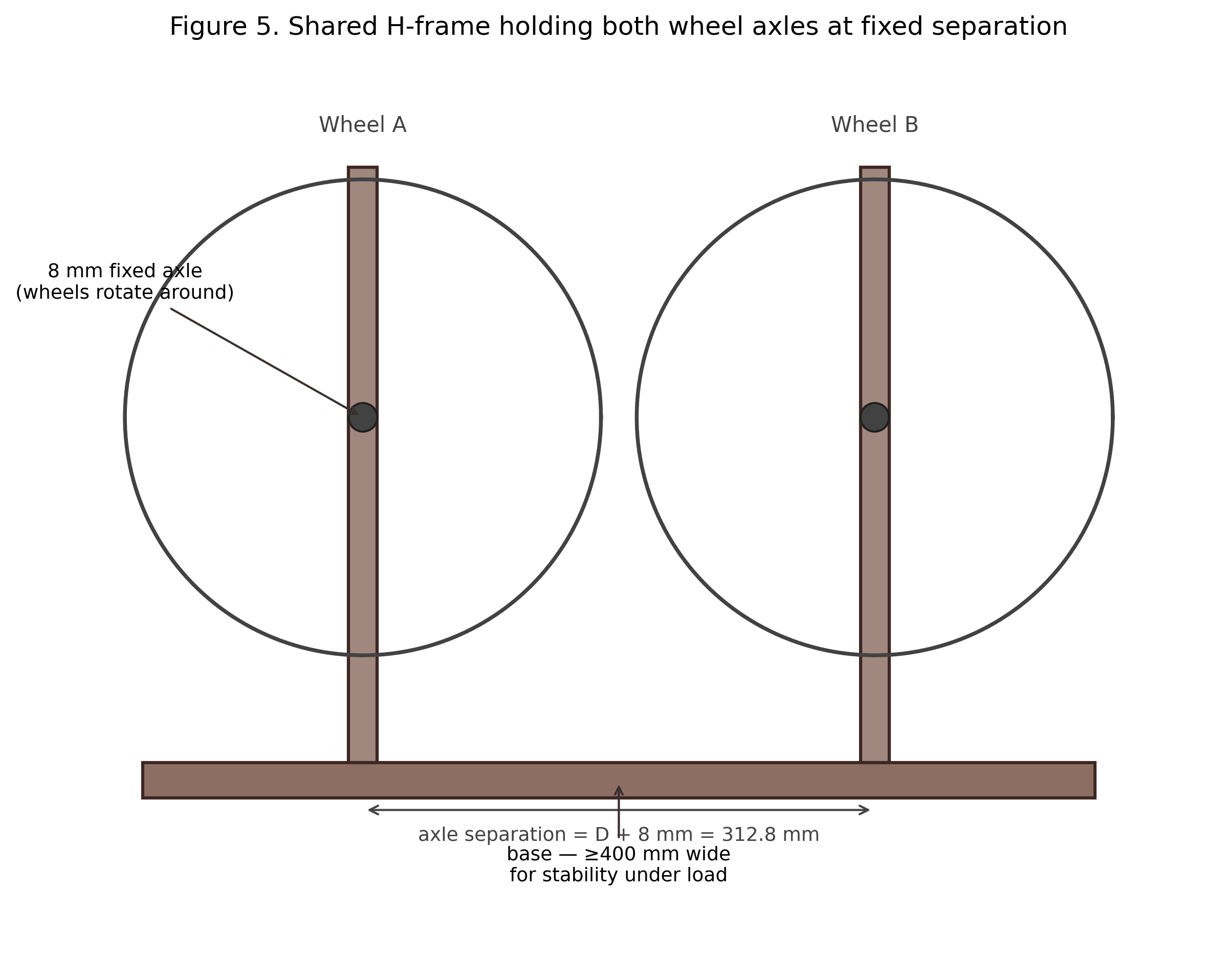
• Type: shared H-frame holding both wheel axles at fixed parallel positions.
• Two vertical side plates connected by a horizontal base.
• Each side plate has fixed 8 mm axle stubs at appropriate height for both wheels.
• Axle separation: WHEEL_OD + WHEEL_MAGNETIC_GAP = 304.8 + 8 = 312.8 mm center-to-center.
• Stability: base width ~400 mm (or wider) to prevent tipping under the loaded mass (~2-3 kg total when fully loaded with both wheels' worth of lead weights).
• Material: TBD: can be MJF-printed alongside the wheels, laser-cut from aluminum flat bar for a more robust feel, or fabricated from wood for prototyping. Frame material does not affect the wheel design.

4.7 Material and print process

• Material: Shapeways Multi Jet Fusion (MJF) PA12 (Nylon 12 powder bed). Selected for:
  • Isotropic strength (no weak layer-line direction, unlike FDM)
  • Tight dimensional tolerance (~0.3 mm on features > 10 mm)
  • Clean surface suitable for press-fits (magnets, bearing) and snap-fits (weight caps)
  • No support material (powder bed self-supports during print)
  • Reasonable cost (~$XXX per wheel-half, to be confirmed via Shapeways quote)
• Minimum walls: 1 mm absolute, 2.5 mm recommended for structural walls in this design.

4.8 Open question: weight measurement

The current parametric model uses placeholder values for the lead weight dimensions:

WEIGHT_L = 38.0 mm    # placeholder, long axis (tangential)
WEIGHT_W = 13.0 mm    # placeholder, short axis (axial / wheel face)
WEIGHT_H = 6.0 mm     # placeholder, thickness (radial / stack direction)

Before final print, the actual weights to be used must be measured (length, width, thickness, and any tapering across the stack). The measurements update three lines in params.py; all derived geometry (pocket dimensions, snap-cap geometry) recomputes automatically.

---

5. Physics of Operation

5.1 Single-wheel dynamics

Each loaded wheel is a physical pendulum about its axle. Let m_total be the total weight mass loaded onto the wheel, and r_offset be the radial distance from the axle to the loaded mass's center of mass. For the dr-Fibonacci distribution with Wheel A configuration [1, 1, 2, 3, 5, 8, 4, 3, 7, 1, 8, 9] (weight counts at 12 stations), the center-of-mass offset is computed by summing the position vectors of each station weighted by its weight count.

At equilibrium, the heaviest side of the wheel hangs at the bottom. Small displacements θ from this equilibrium produce restoring torque τ ≈ -m_total g r_offset θ, giving simple harmonic oscillation with angular frequency

ω_single = √(m_total g r_offset / I_wheel)

where I_wheel is the wheel's moment of inertia about the axle (wheel structure plus loaded weights). For a 12-inch wheel with 1/2-oz weights and the Fibonacci distribution, order-of-magnitude estimates are: m_total ≈ 750 g (fully loaded), r_offset ≈ 50–80 mm, I_wheel ≈ 0.05–0.1 kg·m². This gives ω ≈ 1–3 rad/s, or oscillation period T ≈ 2–6 s. Quantitative measurement is left for the prototype phase.

5.2 Coupled dynamics

The two wheels are magnetically coupled. The coupling can be modeled as a torsional spring between the two wheel angles θ_A and θ_B:

τ_coupling = -K_mag (θ_A + θ_B - φ_offset)

where K_mag is the effective magnetic torsional stiffness (depends on magnet strength, gap, geometry: order 0.1–1.0 N·m/rad for N52 magnets at 8 mm gap) and φ_offset is the equilibrium phase relationship set by initial polarity alignment. The θ_A + θ_B form (rather than θ_A - θ_B) reflects the counter-rotational coupling: when wheel A rotates clockwise, wheel B rotates counter-clockwise, so their angles change in opposite directions.

The equations of motion for the two-wheel system are:

I_A θ̈_A = -m_A g r_A sin(θ_A) - K_mag (θ_A + θ_B - φ_offset) - γ_A θ̇_A
I_B θ̈_B = -m_B g r_B sin(θ_B) - K_mag (θ_A + θ_B - φ_offset) - γ_B θ̇_B

where γ_A, γ_B are damping coefficients (bearing friction, magnetic coupling losses, air drag).

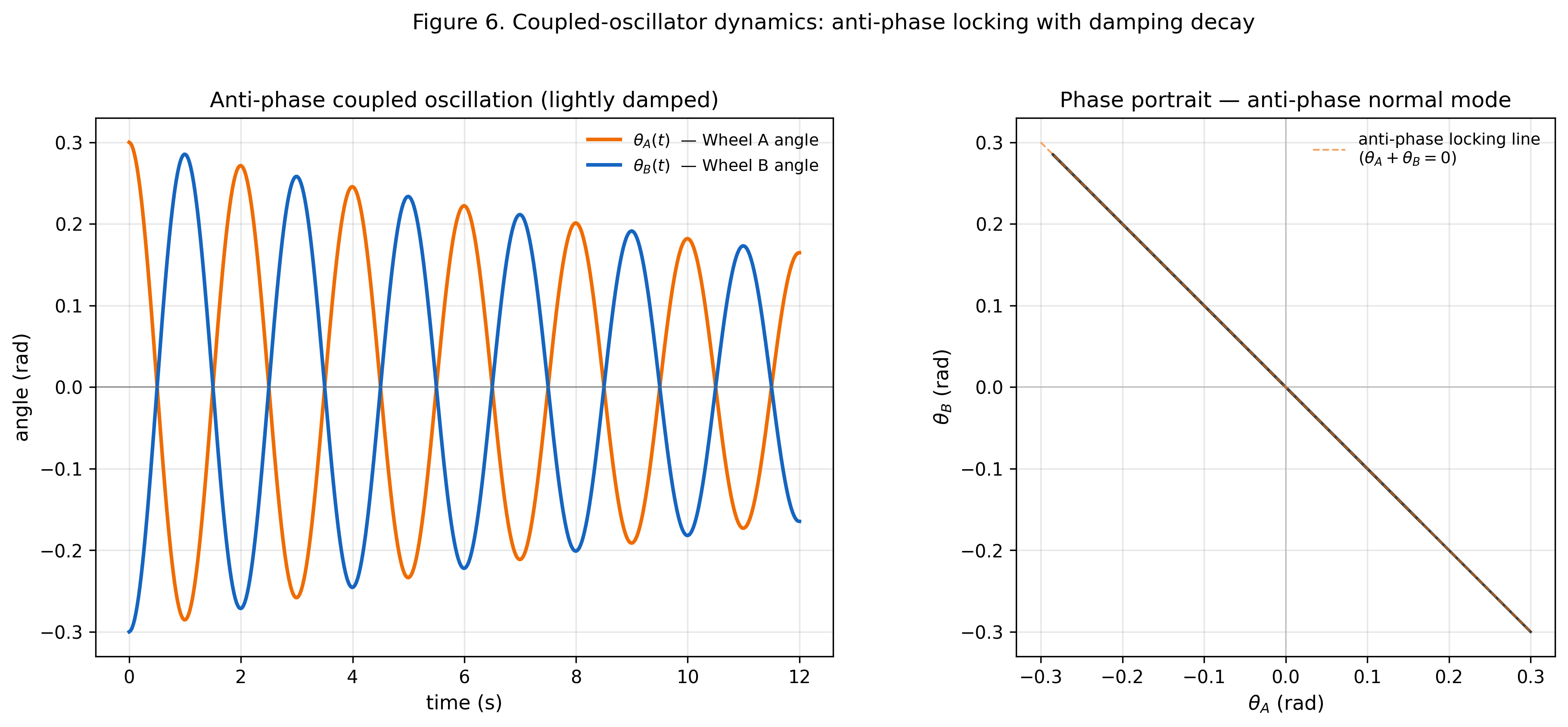
For the symmetric case (I_A = I_B, m_A r_A = m_B r_B, γ_A = γ_B) (which is the design condition for the Fibonacci wheel pair) the coupled system has two normal modes:

• In-phase mode: θ_A + θ_B = 2 θ̄. Frequency unaffected by coupling.
• Anti-phase mode: θ_A - θ_B. Frequency increased by coupling.

In our counter-rotational geometry, the design intent is anti-phase oscillation (wheels rotating in opposite directions), with the magnetic coupling enforcing phase lock.

5.3 Phase locking and Huygens synchronization

Under any perturbation that breaks initial symmetry (including the asymmetric mass distribution itself) the system enters coupled motion. The magnetic coupling enforces phase relationship between the wheels; small initial frequency mismatches are washed out by the coupling for sufficiently large K_mag. The system locks into a stable counter-rotational mode characterized by anti-phase oscillation.

The asymmetric pair-summing structure (Wheel A heavier than Wheel B at some angular positions, lighter at others) provides the driver for sustained motion: at any angular position where Wheel A is heavier, its gravitational torque drags both wheels through the magnetic coupling; the rotation exposes a new pair of stations, possibly with the imbalance reversed; the wheels then "take turns" being the dominant side. This produces sustained rhythmic oscillation as long as input energy or stored momentum exceeds the dissipation rate.

5.4 Why the device "looks like perpetual motion"

The system has a high quality factor Q when bearing friction is low and magnetic-coupling losses are minimized. Q is the ratio of energy stored to energy dissipated per cycle:

Q = ω · E_stored / P_dissipated

For the infinity wheel, oscillation persistence times of minutes to tens of minutes are plausible with high-quality bearings (608 ABEC-7 or ceramic), translating to many hundreds or thousands of oscillation cycles before observable amplitude decay. This is what produces the visual impression of perpetual motion: the casual observer sees a wheel that has been spinning for what seems like an indefinite duration. Careful measurement reveals slow exponential decay, the device is dissipative, just slow about it.

This is consistent with the lineage of overbalanced wheel demonstrations described in §2.3. The infinity wheel does not exit this category; it merely provides a particularly clean, mathematically derived realization.

5.5 Damping mechanisms

Damping in the device comes from:

1. Bearing friction: typically the dominant loss term. Mitigated by high-quality bearings (ABEC-7+, ceramic ball materials, dry / low-viscosity lubricant).
2. Magnetic coupling losses: eddy currents in any conductive material near the magnetic coupling region; hysteresis in the magnets themselves (negligible for N52). Mitigated by avoiding metal frame parts near the rim.
3. Air drag: small at the rotational speeds expected (well below 1 rev/s), but non-zero. Cannot be reduced without operating in vacuum.

The empirical behavior of the v1 prototype (§7) suggests the device can already operate in a regime where these losses are subordinate to the energy stored in the asymmetric mass; quantitative measurement of Q is a target for early v2 testing.

5.6 What this device does NOT claim

For clarity:

• Not perpetual motion. The device is dissipative. With no input energy, it eventually stops.
• Not over-unity. The device returns less energy than is put in.
• Does not violate thermodynamics. First law (energy conservation) and second law (entropy increase) both apply.
• Does not require new physics. Standard Newtonian mechanics with magnetic coupling and dissipation accounts for all expected behavior.

The device is a demonstration of well-understood physics (asymmetric-mass coupled oscillators) realized with an algebraically clean mass distribution.

---

6. Implementation

6.1 Parametric CAD model

The device is implemented as a parametric CAD model in Python using the CadQuery library. The repository structure:

magnetic_gear/
├── MAGNETIC_GEAR_PROJECT.md   ← internal design brief (engineering details)
├── sequences.py                ← dr-Fibonacci math module (the [Math2026] paper's code)
├── params.py                   ← single source of truth for all dimensions
├── wheel_half.py               ← Phase 1 geometry (single clamshell half → STEP)
├── weight_cap.py               ← Phase 2 geometry (snap-fit cap → STEP)
├── wheel_assembly.py           ← Phase 3 (full-wheel assembly preview)
├── frame.py                    ← Phase 4 (H-frame)
├── assembly.py                 ← Phase 5 (full assembly: 2 wheels + frame + axles)
└── output/                      ← STEP and STL files for each part

All dimensions live in params.py; geometry files import from it. Changing a dimension and re-running regenerates all affected geometry. The output is STEP (preserves B-rep solid geometry, fully editable in Fusion 360 / viaCAD Pro), with STL produced as a print-ready secondary.

6.2 Software prerequisites

Python 3.12 (CadQuery does not support 3.13+ as of this writing)
pip install cadquery

The development environment uses pyenv to manage the Python version and a project-local .venv. See magnetic_gear/README.md for setup instructions.

6.3 Print process

Outsourced to Shapeways for MJF PA12. Submission process:

1. Run the CAD scripts to produce STEP files: python wheel_half.py → output/wheel_half.step, etc.
2. Upload STEP files to Shapeways.
3. Select MJF PA12 as material.
4. Verify wall-thickness and minimum-feature warnings are clear.
5. Order: 2× wheel halves (forming one wheel), 24× snap caps (12 per wheel × 2), 1× frame, 1× set of clamshell bolts.

For a two-wheel device: order quantities double (4× wheel halves, 48× snap caps).

6.4 Configuration loading

Once the wheels are printed and assembled with bearings and magnets, they are configured by inserting the appropriate number of lead weights at each station. For the Fibonacci wheel pair (ACTIVE_CONFIG = "fibonacci", SPECIAL_PAIR_MODE = SPECIAL_LOAD_18):

Wheel A station weights (12 stations, in order):  1, 1, 2, 3, 5, 8, 4, 3, 7, 1, 8, 9
Wheel B station weights (12 stations, in order):  8, 8, 7, 6, 4, 1, 5, 6, 2, 8, 1, 9

For SPECIAL_PAIR_MODE = SPECIAL_EMPTY_0, the final 9 in each wheel's sequence becomes 0 (the special-pair stations are emptied).

For the lucas_like and third configurations, the corresponding sequences are generated by WHEEL_CONFIGS in params.py.

6.5 Build cost estimate

(Placeholder, to be updated when Shapeways quote is obtained.)

Item	Quantity	Approx. cost
MJF PA12 wheel halves (1 wheel)	2	$XXX
Snap caps	24	$XX
608 bearings	2 (one per wheel)	$5
N52 disc magnets, 12 mm × 4 mm	24 (one per station × 2 wheels)	$20
8 mm steel axles + frame hardware	1 set	$20
Lead tire weights (1/2 oz, ~150 segments needed)	1 strip	$10
MJF or laser-cut frame	1	$50
Total estimated		~$XXX

---

7. Empirical Observations from a v1 Prototype

A v1 single-wheel prototype was constructed previously (predating this paper's two-wheel design). The v1 wheel embodied a single permutation of the dr-Fibonacci structure (one of the six "wheel N" variants in the predecessor infinity_wheel_v1/ directory).

Qualitative observations from the v1 prototype:

• Sustained rhythmic oscillation under minimal frictional input. The wheel was supported on a held pencil acting as an axle (about as low-friction as can be improvised) and "got into a rhythm" with characteristic period determined by the asymmetric mass distribution. Oscillation persisted for many cycles before observable decay.

• Sync-like behavior in the single-wheel case. Even without explicit coupling to a second wheel, the asymmetric distribution produced a stable oscillation period that the wheel "found" and maintained.

• Bearing friction is the dominant loss term. When bearing friction was minimized (by the pencil-axle expedient), oscillation persistence was substantially longer than with conventional support arrangements.

These observations confirm the design's high-Q regime claim and motivate quality bearing selection for the v2 build (608 standard as a baseline; ABEC-7 or ceramic 608 as upgrades for longer oscillation persistence).

Quantitative measurements (oscillation period, Q factor, decay timescale, sync stability under perturbation) are deferred to the v2 testing phase. Photographs and data from v1 are available in the project repository.

---

8. Discussion

8.1 Educational value

The infinity wheel is a candidate physics demonstration suitable for:

• Physics classrooms: coupled-oscillator dynamics, asymmetric-mass pendulums, magnetic coupling, quality factor and damping.
• Mathematics classrooms: modular arithmetic, Pisano periods, the relationship between recurrence structure and physical realization.
• Museums and science centers: visually compelling demonstration of the illusion of perpetual motion in a clean, mathematically derived form.

The mathematical foundation [Math2026] gives the device an unusual property among physics demonstrations: the design choices are derivable rather than ad hoc. A student who understands the algebra of Z/9Z and Pisano periods can derive the wheel's mass distribution from first principles.

8.2 Possible enhancements (deferred)

The following design enhancements are deferred until v2 baseline behavior is characterized:

• Higher-precision bearings. ABEC-7 or ceramic 608 bearings would reduce dominant friction losses and extend oscillation persistence. Cost: $20–60 per bearing vs. $2 for standard.

• Spring-loaded base. A spring connecting frame to ground could provide elastic energy storage similar to a metronome's escapement, potentially enabling self-resetting oscillation with periodic external input. The builder has expressed interest in this enhancement; it is intentionally deferred until the weights-only baseline is empirically characterized.

• Sensor instrumentation. Optical encoders on the axles, or accelerometers on the rim, would enable quantitative measurement of Q, decay constants, sync dynamics, and frequency response.

• Larger wheels. Scaling up the wheel diameter increases the moment of inertia and gravitational torque proportionally; the dynamics scale predictably. The 12-inch diameter is a Shapeways-friendly compromise; a 24-inch device fabricated from cut sheet stock with separately mounted magnets and weights would be a natural extension.

8.3 Future work: the Flower-of-Life arrangement

The math paper [Math2026] identifies three length-24 orbits, each corresponding to a possible wheel pair. A full realization of the design vision involves three coupled wheel pairs arranged in a "Flower-of-Life" configuration: three magnetic-gear axes at 60° rotations, sharing a common geometric center, with each axis carrying one of the three orbits.

This six-wheel arrangement is left for future work after the single-pair v2 device is built and characterized. The math admits the construction; the engineering complexity (six wheels, three magnetic axes, complex mounting frame) is substantially higher than the present design.

8.4 Limitations and honest framing

The device makes no claims beyond what is presented:

• It is a coupled-oscillator demonstration with mathematically-organized asymmetric mass.
• It exhibits the rhythm-and-sync behaviors expected of such systems.
• It is dissipative, with oscillation duration limited by friction and coupling losses.
• It does not produce energy, violate thermodynamics, or require new physics.

The mathematical structure underlying the design [Math2026] is interesting in its own right and admits broader applications outside this device. See that paper's discussion section. The present paper restricts itself to the mechanical realization.

---

9. References

[Math2026] (Companion math paper, this work), papers/math/canonical.md. Orbital and Multiplicative Structure of Digital-Root Fibonacci Sequences. In preparation, 2026.

[PRK01] A. Pikovsky, M. Rosenblum, and J. Kurths. Synchronization: A Universal Concept in Nonlinear Sciences. Cambridge University Press, 2001. ISBN 978-0521592857.

[Atallah2001] K. Atallah and D. Howe. A novel high-performance magnetic gear. IEEE Transactions on Magnetics 37 (2001), no. 4, 2844–2846.

[Bha12] Bhāskara II. Siddhānta-Śiromaṇi. 12th century. Historical reference for the original overbalanced-wheel concept; multiple modern translations.

[Huy65] C. Huygens. Letter to the Royal Society. 1665. Original report of coupled-pendulum synchronization observation.

[MJFspec] Shapeways / HP Multi Jet Fusion (MJF) PA12 design guidelines. https://www.shapeways.com/materials/multi-jet-fusion-plastic.

[CQ] CadQuery: a Python library for parametric CAD. https://cadquery.readthedocs.io.

[OEIS] N. J. A. Sloane et al. The On-Line Encyclopedia of Integer Sequences. https://oeis.org. Sequence references via [Math2026].

---

Appendix A. Reproducibility checklist

To reproduce this device:

1. Clone the project repository.
2. Set up Python 3.12 via pyenv: pyenv install 3.12.13; pyenv local 3.12.13.
3. Create venv and install CadQuery: python -m venv .venv && source .venv/bin/activate && pip install cadquery.
4. Measure your lead tire weights and update magnetic_gear/params.py: WEIGHT_L, WEIGHT_W, WEIGHT_H.
5. Choose configuration: ACTIVE_CONFIG = "fibonacci" (or "lucas_like" or "third"); SPECIAL_PAIR_MODE = SPECIAL_LOAD_18 (or SPECIAL_EMPTY_0).
6. Generate STEP files: python wheel_half.py, python weight_cap.py, etc. Outputs in magnetic_gear/output/.
7. Visually verify in Fusion 360 / viaCAD Pro 14 / online STEP viewer.
8. Submit STEP files to Shapeways for MJF PA12.
9. Source magnets (N52 12 mm × 4 mm), bearings (608), axles (8 mm steel rod), frame hardware, and lead tire weights.
10. Assemble per MAGNETIC_GEAR_PROJECT.md instructions.
11. Configure weights per the active orbit's loading sequence.
12. Mount in frame; release with small initial perturbation; observe.